Checking ADiMat (first order) derivatives for correctness

When computing derivatives with ADiMat you should always test whether the AD derivatives that come out of ADiMat are plausible and correct. This because there are many builtin functions and toolbox functions that ADiMat does not support yet. While you should get an error message or even a runtime error in these cases, this also hinges on the correct configuration for that builtin in our data base of builtins. Specifically, we mark builtin function that we think have a derivative but that we have not implemented yet. So this markation might be wrong or you might just hit a bug in ADiMat.

Methods for checking derivatives are:

comparison of the ADiMat AD derivatives among each other
comparing the AD derivatives against finite differences
comparing the AD derivatives against the complex variables method
comparing the ADiMat AD derivatives against other AD tools

In this notebook we will discuss the first three of these in detail for the case of first order derivatives.

Comparing AD derivatives among each other
Comparing against finite differences
Comparing against the complex variable method
Creating assertions
All of the above in one line

Comparing AD derivatives among each other

ADiMat has three driver functions for AD, which are admDiffFor, admDiffVFor, and admDiffRev. Let's consider the example function polynom:

type polynom

function r = polynom(x, c)
  r = 0;
  powerOfX = 1;
  for i=1:length(c)
    r = r + c(i) * powerOfX;
    powerOfX = powerOfX * x;
  end

This can for example be used to compute a matrix polynomial:

x = magic(3);
c = (1:10) .* 0.1;
z = polynom(x, c);

Now compute the derivatives with all three AD drivers:

adopts = admOptions();
adopts.functionResults = {z}; % for admDiffRev

[JF, zF] = admDiffFor(@polynom, 1, x, c, adopts);

[Jf, zf] = admDiffVFor(@polynom, 1, x, c, adopts);

[Jr, zr] = admDiffRev(@polynom, 1, x, c, adopts);

Now we have three Jacobian matrices that are hopefully identical. We shall check this by computing the relative error using the norm function.

norm(JF - Jf) ./ norm(JF)
norm(JF - Jr) ./ norm(JF)
norm(Jf - Jr) ./ norm(Jf)

ans =

     0


ans =

   3.1911e-17


ans =

   3.1911e-17

As you see, JF and Jf are absolutely identical. This is quite often the case. However the Jacobian computed by the reverse mode driver differs very slightly. The exponent in the relative error, -17, directly tells you the number of digits by which the results coincide. So the results coincide by at least 16 digits, which for all practical purposes means that they are identical, since the precision of double floats is just about that, slightly larger even:

eps

ans =

   2.2204e-16

This example also shows that it is important to use the relative error. The absolute error is much larger in this case, but this is just because the values in the Jacobian are very large:

norm(JF - Jr)
norm(JF)

ans =

   1.4547e-06


ans =

   4.5586e+10

Comparing against finite differences

Finite differences (FD) are an often-used method for numerically approximating derivatives. While it is easy to write your own FD approximation, even easier it is to use the admDiffFD driver that comes with ADiMat, as it comfortably combines the derivatives w.r.t. x and c into a single Jacobian:

[Jd, zd] = admDiffFD(@polynom, 1, x, c, adopts);

In principle you cannot achieve more than half of the machine precision with FD., so in this case the relative error to the AD derivative will be about 1e-8, which is about the square root of eps.

norm(JF - Jd) ./ norm(JF)
sqrt(eps)

ans =

   1.1418e-08


ans =

   1.4901e-08

In practice you must put consideration into using the correct step size, which you can set via the field fdStep of admOptions. The default is actually sqrt(eps), which in many cases works well enough.

Comparing against the complex variable method

The complex variable (CV) method conceived by Cleve Moler et al. is a very interesting method for numerically approximating derivatives. It uses the approximation

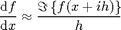$\frac{{\rm d} f}{{\rm d} x} \approx \frac{ \Im\left\{ f(x + ih) \right\} }{ h }$ ,

where $i$ is the imaginary unit and $h$ is some very small value, e.g. 1e-40. There is also a driver for the CV method6 included in ADiMat:

[Jc, zc] = admDiffComplex(@polynom, 1, x, c, adopts);

The CV method is interesting because the derivatives are computed to a very high accuracy, basically up to the machine precision, just as with AD.

norm(JF - Jc) ./ norm(JF)

ans =

   3.2364e-17

Note that CV is only applicable when the function is real analytic, but in our experience a surprisingly large amount of functions that we see actually is. One common issue however is that people tend to use the ctranspose operator ' instead of the transpose operator .' While this does not hurt the results in a real anayltic function, it breaks the CV method. So when the CV method does not give the expected result for you, you first see if this problem affects you.

Creating assertions

In order to turn the insights above into programmatic assertions, it is usually a good idea to be not too strict in our demands. The actual relative errors may differ depending on the function and its arguments, and you don't want your assertions to nag you all the time because of errors that are just slightly larger than expected. We suggest do use assertions like this:

assert(norm(JF - Jr) ./ norm(JF) < 1e-14); % comparing AD vs. AD
assert(norm(JF - Jd) ./ norm(JF) < 1e-5);  % comparing AD vs. FD
assert(norm(JF - Jc) ./ norm(JF) < 1e-14); % comparing AD vs. CV

Especially with the FD method you often have to be extra lenient. When the Jacobians can also become all zero you may run into trouble because of divisions by zero. In these cases you can switch to use the relative-max metric:

type metric

function n = metric(J1, J2)
  maxn = max(norm(J1), norm(J2));
  n = norm(J1 - J2);
  if maxn > 0
    n = n ./ maxn;
  end
end

All of the above in one line

ADiMat provides the function admAllDiff which calls all of the five drivers above and returns the five Jacobians. The calling syntax is similar to the drivers except that it does not accept a seed matrix.

[JF Jf Jr Jd Jc] = admAllDiff(@polynom, x, c, adopts);

On top of that we also provide the function admAllDiffMatrix, which computes the relative errors using the relative-max metric shown above of all results against each other and returns that in a lower triangular five-by-five matrix. This can help a lot in identifying the one who is wrong (if there is just one). You should turn on engineering format, because otherwise everything except the FD-related errors would be shown as zero.

format short e
diffMatrix = admAllDiffMatrix(@polynom, x, c, adopts)